Using an App Registration to Query Log Analytics via Power BI

Power BI is a great tool to visualize data and create effective interactive dashboards and reports. Log Analytics is great to gather and correlate data. Naturally, the two are a great pair. While there isn’t yet a native connector for Log Analytics, you can still pull data by writing a custom M Query in Power BI. Thankfully, with just a couple clicks from Log Analytics, it will generate everything for you so that you don’t need to know M Query to pull data. When doing this, you’ll need to login to Azure using an Organization Account or another interactive login method. But what if you need to have a report that doesn’t require you to login every time? Using an App Registration and authenticating via OAuth can accomplish this, but how do we do that in PowerBI?

Security Disclaimer

The method that I’m going to show you stores the API Key in the dataset/query. This is meant as more of a PoC than something that you would use in any sort of a production environment unless you can protect that data. If you’re putting this report on a PowerBI server, you’ll want to make sure people cannot download a copy of the report file as that would allow them to obtain the API key.

Setup

Before we try to query Log Analytics from Power BI with OAuth, we need to setup an App Registration.

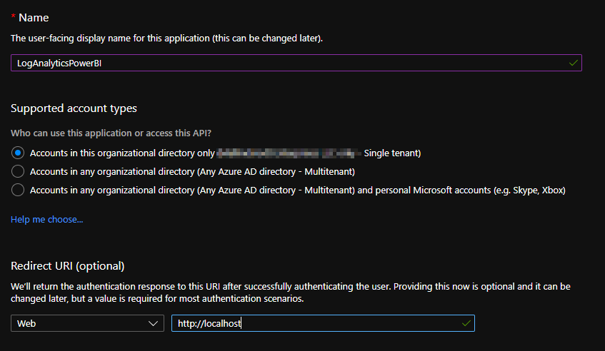
  1. Log into Azure and open App Registrations either from the main portal or via Azure Active Directory. Click on the New Registration button, give it a name and a Redirect URI.

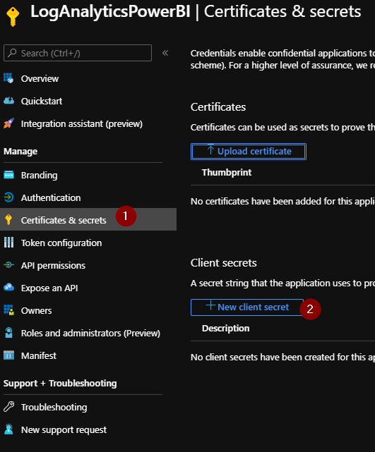
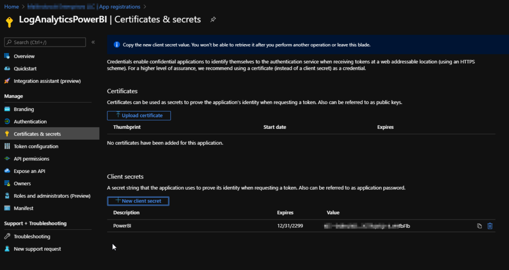
2. Next, generate a new client secret.

Be sure to make note of the client secret as it can not be retrieved once you leave this page.

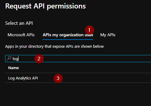
3. Now we need to grant access to the Log Analytics API (Data.Read). To do this, click Add Permission select “APIs my Organization Uses” and search for Log Analytics.

Be sure to select Application Permissions.

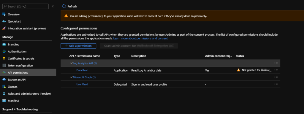
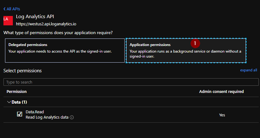
Once you’ve added the permission, you need to grant admin consent to the API to interact on the users behalf.

We now have the App Registration almost ready to go. What we’ve done is grant the App Registration the ability to query the Log Analytics API. What we haven’t don yet is grant it access to our Log Analytics workspaces. We’ll take care of that next.

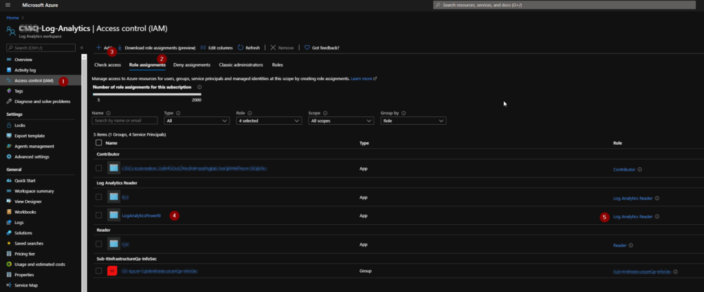
4. Browse to your Log Analytics workspace. We’ll need to add our App Registration to the Log Analytics Reader role. This will grant allow the App Registration the ability to query any table within this workspace. If you want to limit the tables that the app registration is able to query, you will need to define a custom role and assign them to that role instead. I won’t cover creating a custom role in this post, but you can read about how to create a custom role here and see a list of all the possible roles here. You may also want to read through this article to read about the schema for the JSON file that makes up each custom role.

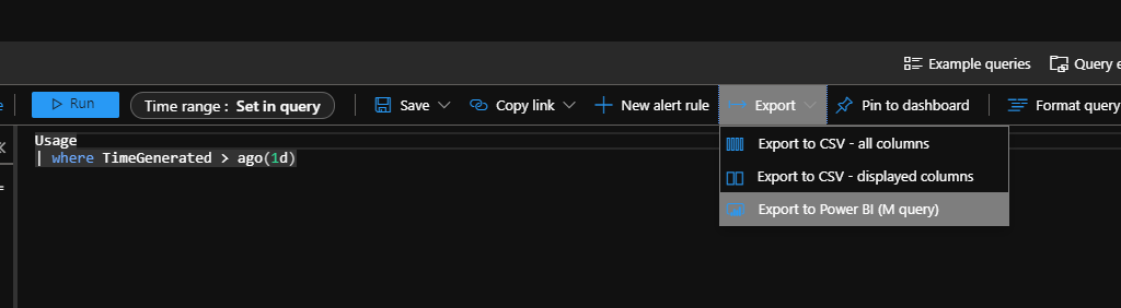
5. Now that the permissions have been granted, let’s run a query. Once you have some results, click on Export and then Export to Power BI (M query). This will download a text file that contains the query. Go ahead an open it up.

The text file will look something like this. If we were to put this into Power BI as is, we could get our data after authenticating with our Organization Account. We’ll take the output and customize it just a bit.

let AnalyticsQuery =
let Source = Json.Document(Web.Contents("https://api.loganalytics.io/v1/workspaces/xxxxxxxx-xxxx-xxxx-xxxx-xxxxxxxxxxxx/query", 
[Query=[#"query"="Usage
| where TimeGenerated > ago(1d)
",#"x-ms-app"="OmsAnalyticsPBI",#"prefer"="ai.response-thinning=true"],Timeout=#duration(0,0,4,0)])),
TypeMap = #table(
{ "AnalyticsTypes", "Type" }, 
{ 
{ "string",   Text.Type },
{ "int",      Int32.Type },
{ "long",     Int64.Type },
{ "real",     Double.Type },
{ "timespan", Duration.Type },
{ "datetime", DateTimeZone.Type },
{ "bool",     Logical.Type },
{ "guid",     Text.Type },
{ "dynamic",  Text.Type }
}),
DataTable = Source[tables]{0},
Columns = Table.FromRecords(DataTable[columns]),
ColumnsWithType = Table.Join(Columns, {"type"}, TypeMap , {"AnalyticsTypes"}),
Rows = Table.FromRows(DataTable[rows], Columns[name]), 
Table = Table.TransformColumnTypes(Rows, Table.ToList(ColumnsWithType, (c) => { c{0}, c{3}}))
in
Table
in AnalyticsQuery

6. Using OAuth is a two step approach. This is commonly known as Two-Legged OAuth where we first retrieve a token, and then use that token to execute our API calls. To get the token, add the following after the first line:

        let ClientId = "xxxxxxxx-xxxx-xxxx-xxxx-xxxxxxxxxxxx",
	ClientSecret = Uri.EscapeDataString("xxxxxxxxxxxxx"),
	AzureTenant = "xxxxxx.onmicrosoft.com",
	LogAnalyticsQuery = "Usage
| where TimeGenerated > ago(1d)
",

	OAuthUrl = Text.Combine({"https://login.microsoftonline.com/",AzureTenant,"/oauth2/token?api-version=1.0"}),
	Body = Text.Combine({"grant_type=client_credentials&client_id=",ClientId,"&client_secret=",ClientSecret,"&resource=https://api.loganalytics.io"}),
	OAuth = Json.Document(Web.Contents(OAuthUrl, [Content=Text.ToBinary(Body)])),

This bit will setup and fetch the token. I’ve split out the Log Analytics query to make it easier to reuse the bit of code for additional datasets. Obviously, you’ll want to put your ClientId, ClientSecret, and Azure Tenant on the first three lines. After that, you’ll want to edit the source line. Change it from:

let Source = Json.Document(Web.Contents("https://api.loganalytics.io/v1/workspaces/xxxxxxxx-xxxx-xxxx-xxxx-xxxxxxxxxxxx/query", 
[Query=[#"query"="Usage
| where TimeGenerated > ago(1d)
",#"x-ms-app"="OmsAnalyticsPBI",#"prefer"="ai.response-thinning=true"],Timeout=#duration(0,0,4,0)])),

to something like this:

Source = Json.Document(Web.Contents("https://api.loganalytics.io/v1/workspaces/xxxxxxxx-xxxx-xxxx-xxxx-xxxxxxxxxxxx/query", 
[Query=[#"query"=LogAnalyticsQuery,#"x-ms-app"="OmsAnalyticsPBI",#"prefer"="ai.response-thinning=true"],Timeout=#duration(0,0,4,0),Headers=[#"Authorization"="Bearer " & OAuth[access_token]]])),

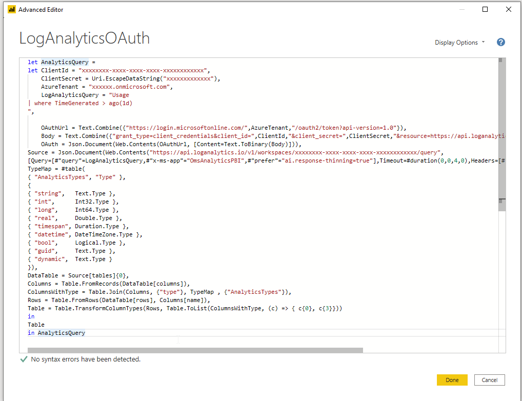
You may notice that we did two things. First, we changed the query to use our variable instead of the text itself. This is done purely to make it easier to re-use the code for additional datasets. The other thing we’ve done is add the Authorization header to the request using the token we obtained from the OAuth line. You should now have something like this:

let AnalyticsQuery =
let ClientId = "xxxxxxxx-xxxx-xxxx-xxxx-xxxxxxxxxxxx",
	ClientSecret = Uri.EscapeDataString("xxxxxxxxxxxxx"),
	AzureTenant = "xxxxxx.onmicrosoft.com",
	LogAnalyticsQuery = "Usage
| where TimeGenerated > ago(1d)
",

	OAuthUrl = Text.Combine({"https://login.microsoftonline.com/",AzureTenant,"/oauth2/token?api-version=1.0"}),
	Body = Text.Combine({"grant_type=client_credentials&client_id=",ClientId,"&client_secret=",ClientSecret,"&resource=https://api.loganalytics.io"}),
	OAuth = Json.Document(Web.Contents(OAuthUrl, [Content=Text.ToBinary(Body)])),
Source = Json.Document(Web.Contents("https://api.loganalytics.io/v1/workspaces/xxxxxxxx-xxxx-xxxx-xxxx-xxxxxxxxxxxx/query", 
[Query=[#"query"=LogAnalyticsQuery,#"x-ms-app"="OmsAnalyticsPBI",#"prefer"="ai.response-thinning=true"],Timeout=#duration(0,0,4,0),Headers=[#"Authorization"="Bearer " & OAuth[access_token]]])),
TypeMap = #table(
{ "AnalyticsTypes", "Type" }, 
{ 
{ "string",   Text.Type },
{ "int",      Int32.Type },
{ "long",     Int64.Type },
{ "real",     Double.Type },
{ "timespan", Duration.Type },
{ "datetime", DateTimeZone.Type },
{ "bool",     Logical.Type },
{ "guid",     Text.Type },
{ "dynamic",  Text.Type }
}),
DataTable = Source[tables]{0},
Columns = Table.FromRecords(DataTable[columns]),
ColumnsWithType = Table.Join(Columns, {"type"}, TypeMap , {"AnalyticsTypes"}),
Rows = Table.FromRows(DataTable[rows], Columns[name]), 
Table = Table.TransformColumnTypes(Rows, Table.ToList(ColumnsWithType, (c) => { c{0}, c{3}}))
in
Table
in AnalyticsQuery

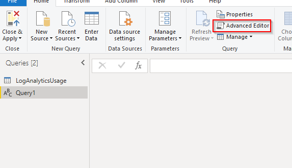
Let’s put that into our query in Power BI. Open Power BI, create a new Blank Query and open the Advanced Editor.

Paste your query and make sure that there are no syntax errors.

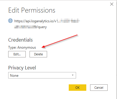
One last thing we will need to do is set our Authentication method to Anonymous. You should be prompted to do so after clicking done, but if not, or you got click happy and dismissed it, you can click on Data Source Settings -> Edit Permissions. If you already have other data sources in your report, be sure to select the one that we just created and change the credentials to Anonymous.

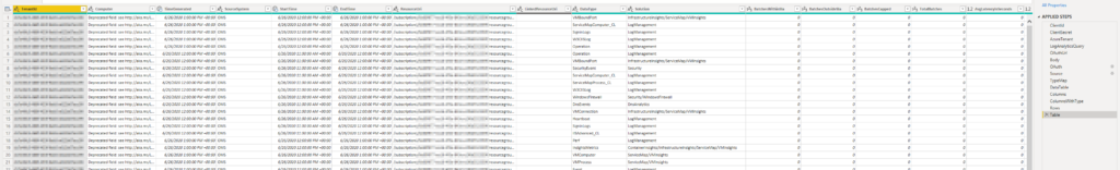
We should now have a preview of our data

Now, if we need to add additional queries, it’s as simple as duplicating the dataset and changing the LogAnalyticsQuery variable on that dataset to the new query.

Building an Azure Connected Fermentation Monitor – Part 1 – The Hardware

Process control is one of the most important aspects of brewing. Sure, I’ve had some great beers that were brewed by people just flopping stuff into a pot. However, without process control, the results are not consistently repeatable. When we talk about process control in brewing, we are usually talking about temperature. Temperature is really everything in beer making and, all else the same, can produce very distinct beers. Temperature can affect just about every characteristic of a batch of beer such as fermentability, mouth feel, flavors, aromas, etc. In this blog post, I’m going to focus on temperature during fermentation and building a controller to do just that. I am going to focus on the hardware here and will do a follow-up post with details about the software. The software that I wrote for this is available on my GitHub space.

How it Works

The fermentation controller works by regulating the temperature during, well, fermentation. There are two outputs on the device, one for a heat source, and one for a cold source. For the cold source, I have a large chest freezer that is large enough to hold four 6 gallon carboys, or a single 60L Spiegel fermenter. When I need to drop the temperature, I trigger the freezer to turn on. Heat is provided using a 100w ceramic reptile bulb. These produce heat, but no light. This is perfect for our use as that’s what we want, heat, no light. By placing everything in a chest freezer, we have a built in cold source, it blocks out light, and it’s insulated so it holds temperature (hot or cold) really well. I’ve been using a Tilt Hydrometer for quite some time along with either their mobile app, or just a Raspberry Pi in a case that I could connect to for viewing the data. With this though, I wanted to have a touchscreen to interact with it and view data or, check on the fermentation away from home.

Parts List

First thing we want to do is gather all of the components that we’ll need for our build. I’ve listed everything out here along with where I bought them and price at time of purchase. There’s a link to the spreadsheet below.

parts
All the parts laid out
  • 14″x11″x5″ Waterproof NEMA Enclosure
  • 4.7k 1/2w Resistor
  • 5v Power Supply
  • Waterproof DS18B20 Temp Sensor
  • Standoffs
  • Data Aquisition Control Plate
  • DAQC Case Plate
  • LED Panel Indicator Lights
  • 3x Extension Cords (two colors)
  • Polycarbonate Buildplate
  • Terminal Strip Blocks
  • Waterproof Cable Glands
  • Insulated Fork Spade Terminal Connectors
  • 7″ Raspberry Pi Touchscreen
  • Raspberry Pi 3b+
  • 2x 20A Solid State Relay
  • Voltage Sensor
  • 3x 15A Clamp Style Current Sensor
  • Waterproof USB (Not Pictured)
  • Waterproof RJ45 (Not Pictured)
  • SSR Heatsink (Not Pictured)
  • Male XLR Panel Mount (Not Pictured)
  • Female XLR Connector (Not Pictured)
  • Tilt Hydrometer (Not Pictured)

Buy List – Total ~$550

The Build

Assembly starts with putting together the Raspberry Pi and DAQC Plate. Sensors and other items can be connected to the Raspberry Pi via the SPI header. The SPI header utilizes a 3.3v signal to determine state and communicate with connected devices. The Pi unfortunately does not have a built in ADC or Analog/Digital Converter. For this, we utilize the DAQC Plate by Pi-Plates to handle all of our sensors and take care of any analog to digital conversions we may need. Pi-Plates are stackable and have a ready built python library that we can use which makes it very attractive in our case. Now, we could also do this build using an arduino or other misc IoT type of board, however, Tilt comes with a ready-built Raspbian based image that is perfect for what we want to do and doesn’t require us to write our own Bluetooth functions.

7″ Touchscreen, Raspberry Pi 3B+, DAQC Plate, Case Plate

Above we have the touchscreen, the Pi, the DAQC Plate, and the Case Plate. The mounting holes on the DAQC plate do not line up with the ones on the Pi, so the Case Plate makes mounting a lot easier and helps protect the contacts and provide support for the hardware.

We start by mounting the first plate to the back of the Touchscreen. We then add a couple of the M2.5 standoffs to then attach the Raspberry Pi
Next, we mount the Pi using some M2.5 screws and connect the screens ribbon cable
We then add some longer standoffs and mount the DAQC Plate. In this photo, I have some of the brass standoffs that I purchased, But I later swapped them out for the PTFE ones that came with the Case Plate as they were just a little too long and I wanted a better mating at the SPI header.
This is what the screen looks like in its assembled form with the Case Plate cover in place.
The inside of the enclosure along with the included accessories.
First thing we’re going to need to do is trim the PC sheet to fit inside. This will act as a non-conductive base to mount all of our components to. It will also allow us to easily remove everything should we need to service something down the road.
A few cuts on the table saw and we have a nice fit with a little bit of space on the sides.
Here I’ve marked all of the standoffs that I will use to mount the PC Sheet to. The standoffs are all varying heights and diameters, but the ones that I colored with a blue sharpie are all the same height and diameter. The one in red protrudes a bit above the rest, so we’ll need to drill a larger hole to accommodate that one so that it doesn’t cause the PC to bend or possibly crack.
I placed the PC sheet inside and transferred the location of the standoffs using the same colors.
I drilled each of them out using a drill press. If you don’t have a drill press, you can use a hand drill, but be careful that you keep the drill steady as PC can be easy to crack.
After drilling, I placed the sheet into the enclosure and made sure everything fit up correctly. Now is the time to make adjustments if you need to.
I drew up a simple wiring diagram to get an idea for how everything would be connected before I started placing components. It’s typically good to have a plan for how things will connect as it can make placement easier if you know where your cables are going to have to go.
Before permanently mounting anything or drilling holes, I dry fit everything together to make sure I had room for everything for all of the components as well as the wires that would be run. The Pi does not mount to the backplate, but I wanted to make sure my components were spaced so that nothing would hit it when the cover was closed.
While the components were in place, I traced out their locations so that I could drill the holes for mounting.
First thing is to drill the mounting holes for the SSRs onto the heatsink. I use a centering punch here to help keep our drill bits from walking when we start to drill. I had a few heatsinks that measured about 9″ x 1″ x 3″ that I had salvaged from some old audio amplifiers many years ago. This project is probably the first (and likely only) time my stockpile of random bits of circuitry was helpful.
With the holes drilled we can tap them to receive our screws. I think I used either M4 or 10-24 screws here.
With the SSR’s mounted, I can mount the other bits to the base board
Last thing to mount is the voltage Sensor
Next, we move on to cutting out the front of the enclosure
After cleaning up the LED holes, I moved on to the hole for the display
These were cut out with a Jigsaw. When the blade is cool, it makes nice clean cuts. However, as the blade heats up, it starts to melt shavings instead of dumping them. If you’re patient, and let the blade cool before continuing to cut, you can avoid this. Patience, unfortunately, is a skill that I lack along with X-Ray vision and super human strength.
To mount the LCD, I use some of the scraps of PC to make strips that will clamp the screen to the front. I put a couple of those soft rubbery feet things on each to add a bit of tension and grip.
An inside look at the screen and LEDs after being mounted
And a view from the front.
Wiring starts with connecting the voltage sensor and 5v power supply. I used a slightly smaller gauge wire here since these two devices have a much lower draw and have their own fuse to prevent over drawing.
To supply power the the Pi and Screen, I took a couple of Micro-USB cables that I had laying around. These will both connect to the 5v power supply. I’m using twist-ties to keep the cables in place for now as I’ll be adding more and will swap them out for cable ties once all the wire is in place. I’ve also drilled and mounted the cable glands and male XLR connector on the bottom of the panel. I didn’t remember to take a picture of that though. I think the drinking started one or two pictures above this.
The red and black wires from the USB cables connect to our output terminals on the power supply
As with most components and sensors, some adjustment is needed out of the box to ensure that our outputs or signals are correct. We just needed to adjust this one a hair.
Before I went any further, I made sure that the Pi booted up and worked with the power supply.
Wiring continues as components are wired up and cables are routed. You can see my input wire in the lower right (black) as well as the two outputs (white) and XLR connector for the temp probe. For the input, I cut the female (receptacle) end off the black extension cord which left me with the plug on the other end that I can plug into the wall to power the unit. For the outputs, I cut about 12″ from the female end and used those as tails to plug the freezer into. The rest of the wire was removed from the outer jacket to wire the internal components.
Another quick boot to make sure we didn’t fry anything and to check our wiring.
Next we add the current sensors. One for the main, and one each for the cold and hot side.
Next, we connect the SSRs to the DAQC plate and wire up the XLR connector. We have to add our 4.7k ohm resistor here to get accurate readings.
Pictures can sometimes be hard to see what connects to what. Hopefully this illustrates it a little bit better. The SSRs connect to the digital outputs on the left. We need to use a jumper here between the first and second to last pin as a safety. Our current and voltage sensors (the signal pin at least) connect to our analog inputs in the lower left. Our temp sensor and the ground for everything except for the SSRs connect to the digital inputs on the lower right.
Remember how I said we have to adjust some components? This is the output from the voltage sensor. This *should* be a nice sine wave. This is an oscilloscope that my Uncle gave me over 20 years ago. I had never used it… Until Now. The only time my reluctance to throw anything away has come in handy.
After adjusting, we now have a clean wave and can take accurate measurements. This adjustment has to be done with the power on, so be careful doing this as you have exposed electrical components. Making contact with the wrong part could damage your equipment or you.
I wrote up a quick python script to check the voltage and amperages. We’re getting readings, although the amperage is off.
Our completed build. S = Set or Target Temperature, V = Value or Current reading, G = Gravity, Delta is the amount above or below the set temperature the unit trigger the cold or heat.
Setting the target temperature
Other setting adjustments along with the ability to reboot or power off the device.

Now you might be wondering about how I got the screen to look the way it does. That’ll be covered in my next blog post, but I have uploaded the source code to GitHub if you want to rummage through it. There’s a couple things we need to do to get it to work from the Pi side, but I’ll cover all of that in the next post. Here’s what our data looks like:

Gravity Readings over the course of a day
Temperature. You can tell where I started cold crashing.